Python for Biomathematics

Artwork by CevRiemann

Overview

Scientific computing software plays a major role in biomathematics for many reasons some of which include:

The complexity of biological systems leads to models or equations that are difficult to work with analytically but can be handled reasonably well by numerical methods.
The need to synthesize theoretical models and data from experiments.
Plots and other visualizations are important for understanding and communicating scientific ideas and results.
Computing allows us to use theoretical models to conduct experiments in silico that would be difficult or impossible to conduct otherwise.

Thus, this course will make use of scientific computing software. Three commonly used free and open-source languages for scientific computing in biomathematics are R, Julia, and Python. In this course, we will mostly use R, but it’s worth knowing at least a little about scientific computing in all three languages as each of them has its own strengths and weaknesses in the context of scientific computing for biomathematics. The goal is not to teach you to become an expert in any of these languages, but rather to become familiar with how to use them to solve some basic problems in biomathematics. Thus, this document is more of a reference than a tutorial.

This page will focus on Python. The other two languages have their own pages:

Each of these pages will have a similar structure to this one. We do not provide details on or even an introduction to the basics of programming or the structure of any of the languages. There are many resources available for learning these things. Instead, we focus on providing some concise examples of the use of these languages for scientific computing in biomathematics. The hope is that the reader will be able to copy and modify these examples to solve their own problems.

The section titles listed in the table of contents for the page should indicate the topics or types of problems we provide examples for. For some of the more involved code, we provide links to additional webpages that provide more details. In some cases, we provide links to potentially helpful videos or web sites where the reader can learn more.

Python

Python is an elegant an mature general-purpose programming language (Van Rossum and Drake 2009). You can learn more about the history of Python here.

Functions and Modules

As in R, most of the algorithms and methods we will want to use in solving problems in biomathematics are implemented as functions in Python. However, base Python contains very few functions useful for mathematics or scientific computing. Most of the functions we will need are contained in modules. A module is a collection of functions and other objects that can be imported into Python. There are many modules available for scientific computing in Python. We will focus on a few of the most commonly used ones such as

NumPy: Numerical Python, offers comprehensive mathematical functions, random number generators, linear algebra routines, Fourier transforms, and more.
SciPy: Scientific Python, provides algorithms for optimization, integration, interpolation, eigenvalue problems, algebraic equations, differential equations, statistics and many other classes of problems.
Matplotlib: Plotting in Python, is a comprehensive library for creating static, animated, and interactive visualizations in Python.
SymPy: Symbolic Python, is a library for symbolic mathematics.
py-pde: py-pde is a python package providing methods and classes useful for solving partial differential equations (PDEs).

One thing that is a little different working in Python (and also Julia) compared to R is that it’s common practice to utilize virtual environments to avoid conflicts between functions and objects from different modules. Environments also help keep track of different versions of the Python interpreter. We will not go into details about how to use environments here, but we will provide some links to resources that explain how to use them.

Envinronment Setup

The most common tool in the scientific community for managing Python environments is Conda. Conda is a package manager that can be used to install Python and other software packages. It can also be used to create and manage virtual environments. Conda is available for Windows, Mac, and Linux. You can download and install Conda from here. To learn about using Conda, see the following video:

Master the basics of Conda environments in Python YouTube video, watch video on YouTube.

The nice thing about working with virtual environments is that we can easily share the environment with others. To do this, we can create a file called environment.yml that contains a list of all the packages we want to install in the environment. For example, the environment.yml file from the GitHub repository will create an environment called biomath_py that contains Python 3.9 and the NumPy, SciPy, Matplotlib, and SymPy modules among others.

Once we have set up and activated the environment, we can import modules and use functions from them. For example, to import the NumPy module and compute $\sin (\frac{π}{4})$ , we can use the following code:

from numpy import sin, pi

sin(pi/4)

0.7071067811865475

Plotting

import matplotlib.pyplot as plt
import numpy as np

plt.rcParams['text.usetex'] = True


x = np.linspace(-2.0, 2.0, 101)
y2 = np.power(x,2)

def f(x):
    return np.power(x,2)

fig, ax = plt.subplots(figsize=(7, 5), tight_layout=True)

ax.set_xlabel(r'\textit{$x$}',fontsize=13)
ax.set_ylabel('\\textit{$y$}',fontsize=13)
ax.set_title(r'$f(x) = x^2$',fontsize=15)
ax.plot(x, f(x))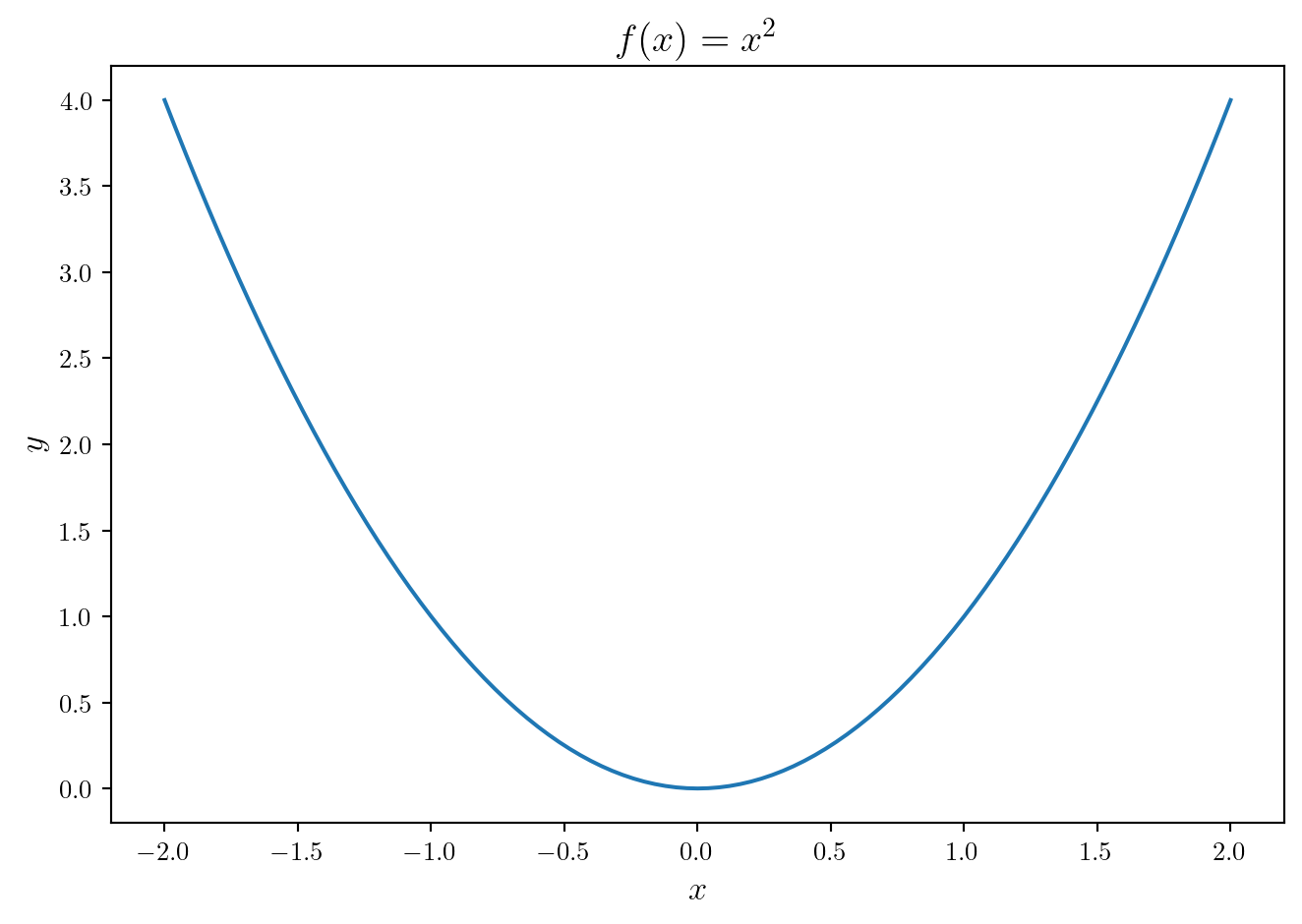

def g(x):
    return np.power(x,3)
  
# Set custom figure size
plt.figure(figsize=(8, 6))

# Plot the curves
plt.plot(x, f(x), label=r'$x^2$', color='steelblue', linewidth=2)
plt.plot(x, g(x), label=r'$x^3$', color='purple', linewidth=2)

# Add labels and title
plt.xlabel(r'$x$',fontsize=13)
plt.ylabel(r'$y$',fontsize=13)
plt.title(r'$f(x) = x^2$',fontsize=13)

# Add legend
plt.legend()

# Show the plot
plt.grid(True)
plt.show()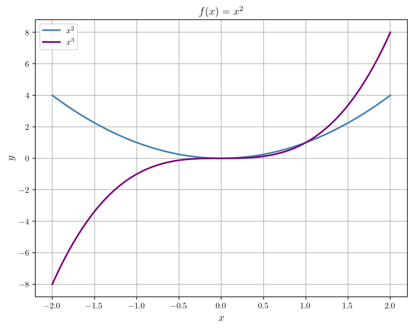

Figure 2: Plot of $f (x) = x^{2}$ and $g (x) = x^{3}$ on same axes.

# Create subplots
fig, (ax1, ax2) = plt.subplots(nrows=1, ncols=2, figsize=(8, 5))

# Plot y = x^2
ax1.plot(x, f(x), color='steelblue', linewidth=2)
ax1.set_title(r'$f(x) = x^2$')
ax1.set_xlabel(r'$x$')
ax1.set_ylabel(r'$y$')
ax1.grid(True)

# Plot y = x^3
ax2.plot(x, g(x), color='purple', linewidth=2)
ax2.set_title(r'$f(x) = x^3$')
ax2.set_xlabel(r'$x$')
ax2.set_ylabel(r'$y$')
ax2.grid(True)

# Adjust layout to prevent overlap
plt.tight_layout()

# Show the subplots
plt.show()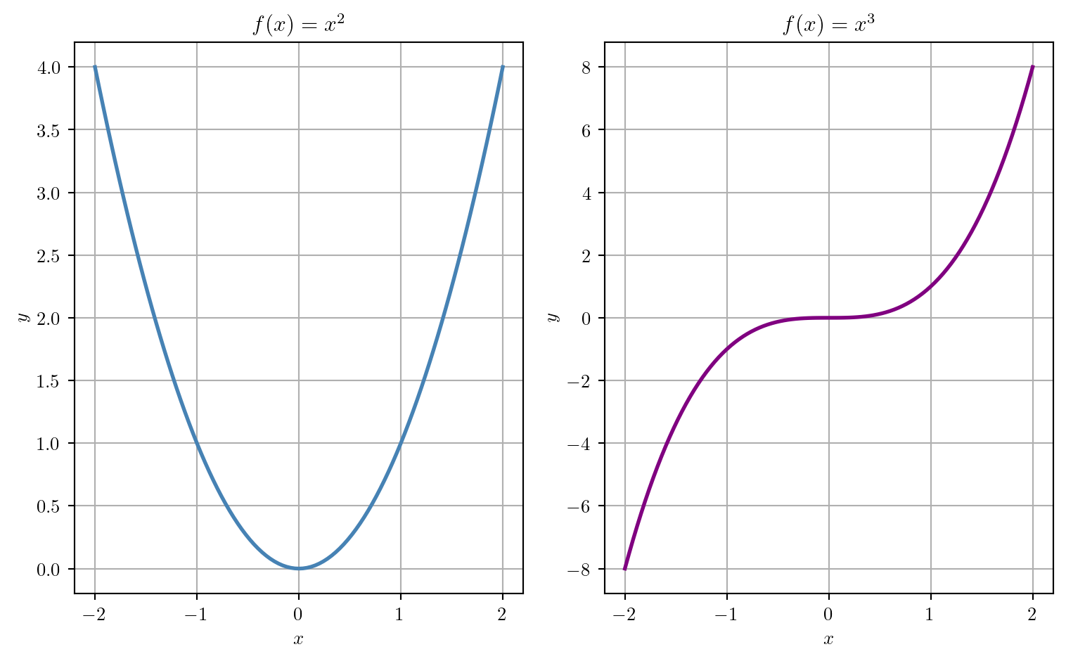

Figure 3: Plot of $f (x) = x^{2}$ and $g (x) = x^{3}$ .

Plotting in Python YouTube video, watch video on YouTube.

Matrices and Linear Systems

import numpy as np
from scipy import linalg

Here’s a vector:

my_vect = np.array([1.0,-1.0,1.0])
print(my_vect)

[ 1. -1.  1.]

Here’s a matrix:

my_matrix = np.array([[1.0, 0.0, -1.0],[3.0, 1.0, 2.0],[-1.0, 1.0, 2.0]])
print(my_matrix)

[[ 1.  0. -1.]
 [ 3.  1.  2.]
 [-1.  1.  2.]]

Here’s the matrix-vector product:

b_vect = my_matrix @ my_vect
print(b_vect)

[0. 4. 0.]

Here’s the determinant of the matrix:

matrix_det = linalg.det(my_matrix)
print(matrix_det)

-4.0

Here are the eigenvalues and eigenvectors of the matrix:

eig_vals, eig_vects = linalg.eig(my_matrix)
print(eig_vals)
print(eig_vects)

[-0.73205081+0.j  2.        +0.j  2.73205081+0.j]
[[ 0.23617375 -0.57735027 -0.49557222]
 [-0.88141242 -0.57735027  0.13278818]
 [ 0.40906493  0.57735027  0.85835626]]

Here’s the solution to the linear system:

x_vect = linalg.solve(my_matrix, b_vect)
print(x_vect)

[ 1. -1.  1.]

To learn more, check out

Linear Algebra in Python with SciPy and NumPy YouTube video, watch video on YouTube.

Root Finding

Root finding is the process of finding one or more values $x$ such that $f (x) = 0$ ¹. A common application of root finding in biomathematics is to find the steady states of a dynamical system.

The scipy.optimize module contains functions for root finding in Python. For example, following code uses the scipy.optimize.root_scalar function to find the roots of the function $f (x) = x^{2} - 1$ on $[- 2, 2]$ .

We start by plotting the function to get an idea of where the roots are located.

import numpy as np
import matplotlib.pyplot as plt

def f(x):
    return x**2 - 1
  
x = np.linspace(-2, 2, 101)

plt.figure(figsize=(8, 6))

plt.plot(x, f(x), color='steelblue', linewidth=2)

plt.xlabel(r'$x$',fontsize=13)

plt.ylabel(r'$y$',fontsize=13)

plt.title(r'$f(x) = x^2 - 1$',fontsize=13)

plt.grid(True)

plt.show()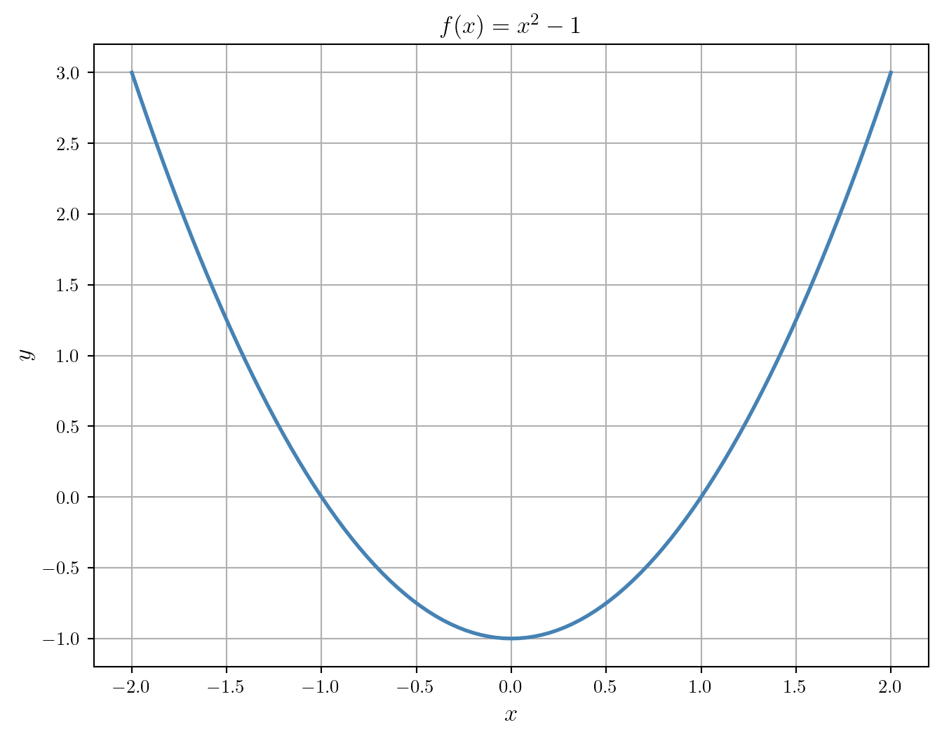

Now, let’s compute the roots:

from scipy import optimize

def f(x):
    return x**2 - 1
  
root_1 = optimize.root_scalar(f, bracket=[-2, 0])
root_2 = optimize.root_scalar(f, bracket=[0, 2])

print(root_1.root)
print(root_2.root)

-1.0
1.0

Finally, let’s add the roots to the plot:

plt.figure(figsize=(8, 6))

plt.plot(x, f(x), color='steelblue', linewidth=2)

plt.plot([root_1.root, root_2.root], [0, 0], 'o', color='purple', markersize=10)

plt.xlabel(r'$x$',fontsize=13)

plt.ylabel(r'$y$',fontsize=13)

plt.title(r'$f(x) = x^2 - 1$',fontsize=13)

plt.grid(True)

plt.show()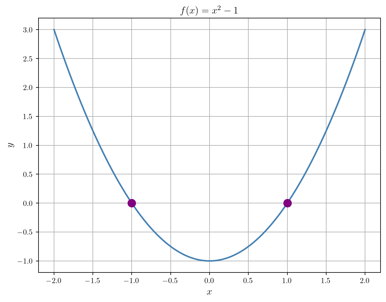

Here’s an example of using the scipy.optimize.root function to find a of root of the system of equations $f (x, y) = (x^{2} + y^{2} - 1, x^{2} - y^{2} + 0.5)$ :

def f(x):
    return [x[0]**2 + x[1]**2 - 1, x[0]**2 - x[1]**2 + 0.5]
  
f_roots = optimize.root(f, [1.0, 1.0])

print(f_roots.x)

[0.5       0.8660254]

Optimization

Optimization is the process of finding the extrema, that is, maximum or minimum value of a function. A common application of optimization in biomathematics is to estimate parameters for a mathematical model to fit data. One of the major challenges in such optimization problems is the potential for multiple local extrema. Here, introduce the use of basic optimization methods implemented in Python. Additional details, examples, and applications will be covered in course lectures.

The scipy.optimize module contains functions for optimization in Python. For example, following code uses the scipy.optimize.minimize function to find the minimum of the function $f (x) = x^{2} - 1$ on $[- 2, 2]$ .

We start by plotting the function to get an idea of where the minimum is located.

import numpy as np
import matplotlib.pyplot as plt

def f(x):
    return x**2 - 1
  
x = np.linspace(-2, 2, 101)

plt.figure(figsize=(8, 6))

plt.plot(x, f(x), color='steelblue', linewidth=2)

plt.xlabel(r'$x$',fontsize=13)

plt.ylabel(r'$y$',fontsize=13)

plt.title(r'$f(x) = x^2 - 1$',fontsize=13)

plt.grid(True)

plt.show()

Now, let’s compute the minimum:

from scipy import optimize

def f(x):
    return x**2 - 1

min_result = optimize.minimize(f, 0.2)

print(min_result.x)

[4.28408381e-09]

Finally, let’s add the minimum to the plot:

plt.figure(figsize=(8, 6))

plt.plot(x, f(x), color='steelblue', linewidth=2)

plt.plot(min_result.x, f(min_result.x), 'o', color='purple', markersize=10)

plt.xlabel(r'$x$',fontsize=13)

plt.ylabel(r'$y$',fontsize=13)

plt.title(r'$f(x) = x^2 - 1$',fontsize=13)

plt.grid(True)

plt.show()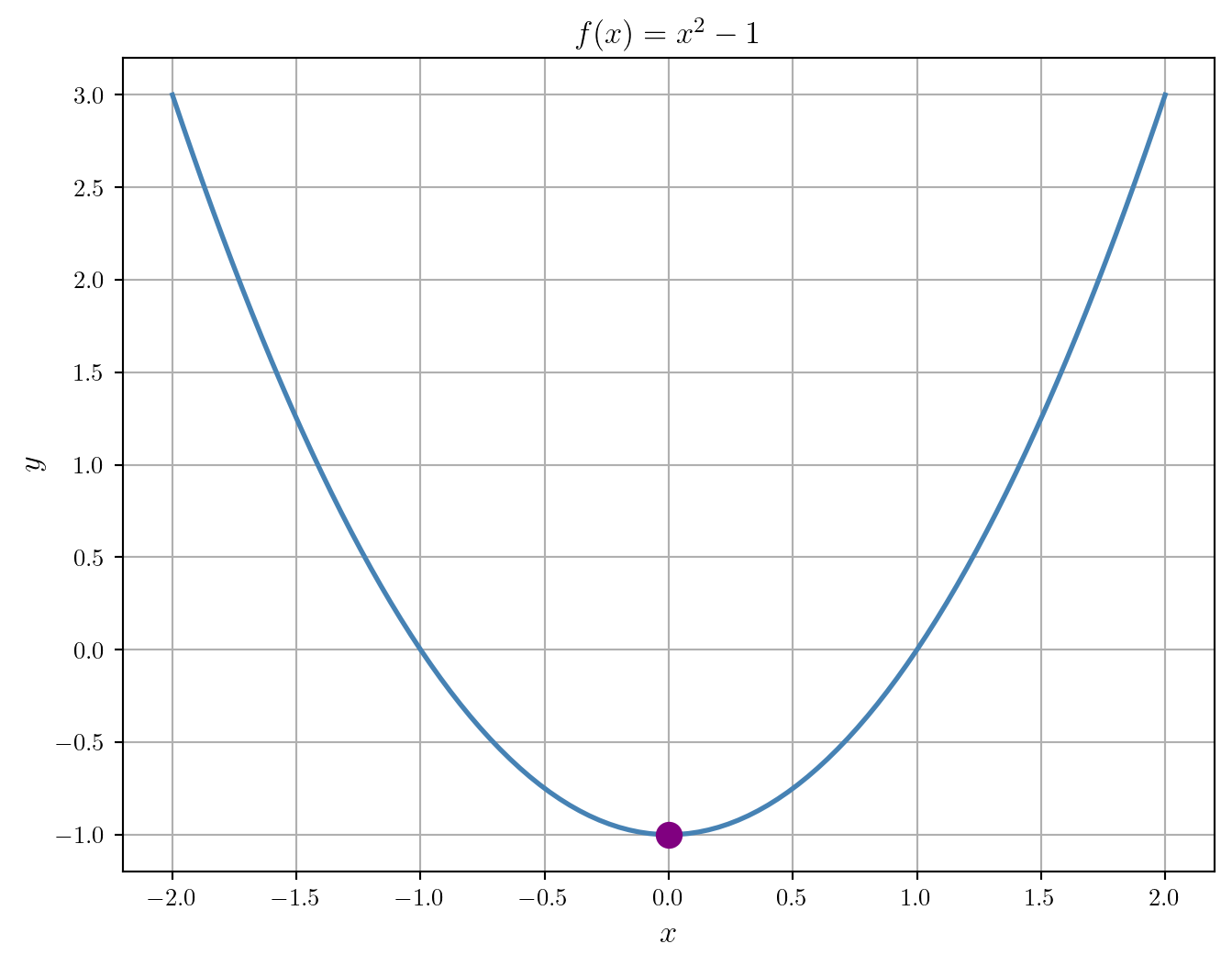

Here’s an example of using the scipy.optimize.minimize to find the minimum of the function $f (x, y) = x^{2} + y^{2} - 1$ :

def f(x):
    return x[0]**2 + x[1]**2 - 1


min_result = optimize.minimize(f, [1.0, 1.0])

print(min_result.x)

[-8.14241718e-09 -8.14241718e-09]

Differential Equations and Dynamical Systems

In this section, we provide an overview and links to detailed examples of the numerical solution of initial value problems (IVPs) for ordinary differential equations (ODEs). Additionally, the linked examples illustrate computations and visualizations of the phase plane and phase portraits for systems of ODEs. For the numerical solution of ODEs, we will use the solve_ivp from the scipy.integrate module.

Briefly, most implementations of numerical methods for IVPs for ODEs require the user to define a function that returns the value of the derivative of the solution at a given time, that is, the right hand side of the ODEs. Further, the user must specify an initial condition, a time interval over which to solve the ODEs, and the values of any parameters.

View webpage with basic examples

Partial Differential Equations

Partial differential equations (PDEs) generalize ordinary differential equations (ODEs) to allow for solutions that are functions of two or more variables. Typically, in the context of biomathematics, the variables represent time and spatial coordinates. Thus, PDEs allow us to model how a biological systems change in both time and space. The examples we will see in this course will mostly be convection-diffusion type equations or systems of such equations. These PDEs have the form

$\frac{\partial c}{\partial t} = \nabla \cdot (D \nabla c - v c) + R$

Special cases include diffusion equations of which the heat equation

$\frac{\partial c}{\partial t} = D \nabla^{2} c$

is a special case. In one dimension, the heat equation is

$\frac{\partial c}{\partial t} = D \frac{\partial^{2} c}{\partial x^{2}}$

Often, in order to have a complete model, we need to specify both initial conditions and boundary conditions for the PDE problem. For example in the case of the one-dimensional heat equation, we might specify the initial temperature distribution $c (x, 0)$ and the values of the flux at the boundaries, that is $\frac{\partial c}{\partial x} (0, t)$ and $\frac{\partial c}{\partial x} (L, t)$ for $t > 0$ .

There are many approaches to the numerical solution of PDEs. We will focus on the method of lines which discretizes the spatial domain and then uses ODE solvers such as those we previously described to solve the resulting system of ODEs.

For Python, the py-pde module is available to facilitate the implementation of the method of lines for PDEs. The following links illustrate the use of this package:

Numerical solution of the heat equation in Python - this page demonstrates using the py-pde module to obtain and visualize numerical solutions for the heat equation in one dimension.

Random Variables

While MATH 463 primarily focuses on deterministic models, stochastic models are also important in biomathematics, see for example (Allen 2011). We won’t cover stochastic models in the course but will have a few occasions where it will be useful to add some stochasticity to a deterministic model. Many different probability distributions are available in Python through the scipy.stats module. In this section, we introduce some functions associated with distributions and random sampling. Primarily, we focus on sampling from a distribution and accessing the probability density or probability mass function for a distribution. Further, we will demonstrate the main functions for the normal distribution and the binomial distribution. Working with other distributions is handled similarly. Additional details, examples, and applications will be covered in course lectures.

Binomial Distributions

Recall that a binomial distribution is a discrete probability distribution that models the number of successes in a sequence of $n$ independent experiments, each asking a yes–no question, and each with its own Boolean-valued outcome: success/yes/true/one (with probability $p$ ) or failure/no/false/zero (with probability $q = 1 - p$ ). A single success/failure experiment is also called a Bernoulli trial or Bernoulli experiment and a sequence of outcomes is called a Bernoulli process; for a single trial, i.e., $n = 1$ , the binomial distribution is a Bernoulli distribution. The probability of outcomes for a binomial random variable are given by the binomial probability mass function for:

$f (k, n, p) = Pr (k; n, p) = Pr (X = k) = (\binom{n}{k}) p^{k} (1 - p)^{n - k}$

where $k$ is the number of successes, $n$ is the number of trials, and $p$ is the probability of success in each trial.

Let’s work with a binomial distribution in Python. First, we import the binom function from the scipy.stats module:

from scipy.stats import binom

Now, let’s define a binomial random variable with $n = 10$ and $p = 0.5$ :

n = 10
p = 0.5
binom_rv = binom(n,p)

We can now access the mean, variance, and standard deviation of the random variable:

binom_rv.mean()

5.0

binom_rv.var()

2.5

binom_rv.std()

1.5811388300841898

Notice that the mean is $n p$ and the variance is $n p (1 - p)$ , as expected. Further, the standard deviation is the square root of the variance:

np.sqrt(2.5)

1.5811388300841898

We can work with the probability mass function as follows:

binom_rv.pmf(4)

0.20507812499999997

Figure 4 displays the probability mass function for a binomial random variable with $n = 10$ and $p = 0.5$ .

# Figure size
plt.figure(figsize=(8, 6))

# Outcome values
x = np.arange(0,11)
# Plot the bar plot
plt.bar(x, binom_rv.pmf(x), color='steelblue', align='center')

# Customize the plot
plt.title('Binomial Distribution PMF')
plt.xlabel('Number of Successes')
plt.ylabel('Probability')
plt.xticks(x)
plt.text(8,0.21,r'$n=10, p =0.5$', fontsize=13)

# Display the plot
plt.show()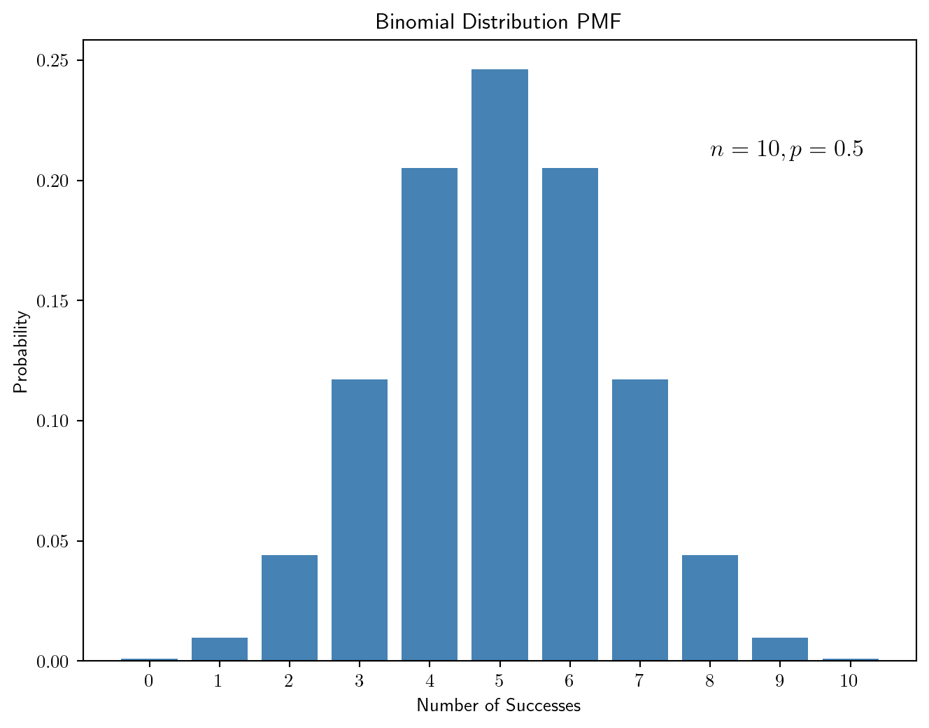

Figure 4: Probability mass function for a binomial random variable with n=10 and p=0.5.

We can also sample from the binomial distribution:

binom_rv.rvs(size=10)

array([8, 3, 5, 6, 6, 5, 5, 5, 6, 6])

Let’s generate a large number of samples and plot a histogram of the results, see Figure 5.

# Figure size
plt.figure(figsize=(8, 6))

# Generate 1000 samples
samples = binom_rv.rvs(size=1000)

# Plot the histogram
plt.hist(samples, bins=10, histtype='bar', ec="black", color='steelblue', align='left', rwidth=1)

# Customize the plot
plt.title('Binomial Distribution Samples')
plt.xlabel('Number of Successes')
plt.ylabel('Count')
plt.xticks(x)
plt.text(7.5,200,r'$n=10, p =0.5$',fontsize=13)
# Display the plot
plt.show()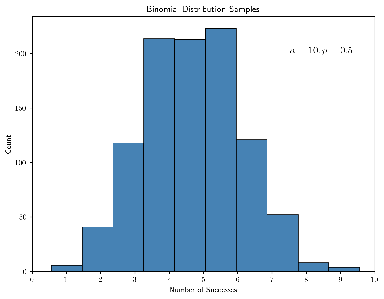

Figure 5: Histogram of 1000 samples from a binomial random variable with n=10 and p=0.5.

Normal Distributions

Recall that a normal distribution is a continuous probability distribution that is symmetric about the mean, showing that data near the mean are more frequent in occurrence than data far from the mean. In graph form, normal distribution will appear as a bell curve. Normal distributions are extremely important in statistics and are often used in the natural and social sciences to represent real-valued random variables whose distributions are not known. A random variable with a Gaussian distribution is said to be normally distributed and is called a normal deviate. The probability that a normal random variable with mean $μ$ and variance $σ^{2}$ has a value between $a$ and $b$ is given by the definite integral of a normal density function defined by:

$f (x ∣ μ, σ^{2}) = \frac{1}{\sqrt{2 π σ^{2}}} \exp (- \frac{(x - μ)^{2}}{2 σ^{2}})$

The parameter $σ$ is called the standard deviation.

Let’s work with a normal distribution in Python. First, we import the norm function from the scipy.stats module:

from scipy.stats import norm

Now, let’s define a normal random variable with $μ = 5$ and $σ = 1.5$ :

mu = 5
sigma = 1.5
norm_rv = norm(mu,sigma)

Figure 6 displays the probability density function for a normal random variable with $μ = 5$ and $σ = 1.5$ .

# Figure size
plt.figure(figsize=(8, 6))

# Outcome values
x = np.linspace(0,10,100)
# Plot the pdf
plt.plot(x, norm_rv.pdf(x), color='steelblue', lw=2)

# Customize the plot
plt.title('Normal Distribution PDF')
plt.xlabel(r'$x$',fontsize=13)
plt.ylabel(' ')
plt.text(1,0.25,r'$\mu=5, \sigma =1.5$', fontsize=13)

# Display the plot
plt.show()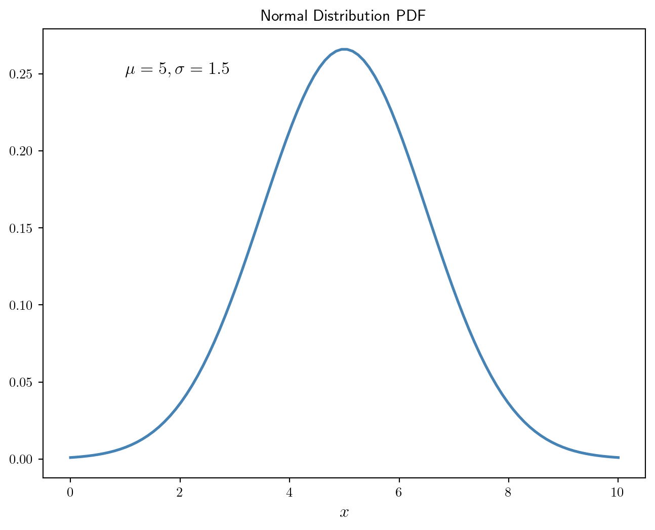

Figure 6: Probability density function for a normal random variable with $μ = 5$ and $σ = 1.5$ .

We can sample from a normal distribution with $μ = 5$ and $σ = 1.5$ as follows:

norm_rv.rvs(size=10)

array([4.89903623, 6.94486314, 3.73359347, 4.51750146, 4.02969902,
       4.139107  , 5.04691272, 3.89045516, 4.7942513 , 4.91356273])

Let’s generate a large number of samples and plot a histogram of the results, see Figure 7.

# Generate samples
r = norm_rv.rvs(size=1000)

# Create figure
fig, ax = plt.subplots(1, 1)

# Outcome values
x = np.linspace(0,10,100)
# Plot the pdf
ax.plot(x, norm_rv.pdf(x), color='steelblue', lw=2)
# Plot the histogram
ax.hist(r, density=True, bins='auto', histtype='stepfilled', alpha=0.2)
# Customize the plot
plt.title('Normal Distribution PDF')
plt.xlabel(r'$x$',fontsize=13)
plt.ylabel(' ')
plt.text(1,0.25,r'$\mu=5, \sigma =1.5$', fontsize=13)

# Display the plot
plt.show()

Figure 7: Histogram of 1000 samples from a normal random variable with $μ = 5$ and $σ = 1.5$ . Here, we’ve also plotted the corresponding probability density function.

Symbolic Math

References

Allen, Linda J. S. 2011. An Introduction to Stochastic Processes with Applications to Biology. Second. CRC Press, Boca Raton, FL. https://mathscinet.ams.org/mathscinet-getitem?mr=2560499.

Van Rossum, Guido, and Fred L. Drake. 2009. Python 3 Reference Manual. Scotts Valley, CA: CreateSpace.

Expand for Session Info

Show the code

import sys
import numpy as np
import scipy as sp
import matplotlib as mpl
print("Python version:", sys.version)
print('\n'.join(f'{m.__name__}=={m.__version__}' for m in globals().values() if getattr(m, '__version__', None)))

Python version: 3.8.18 | packaged by conda-forge | (default, Oct 10 2023, 15:46:56) 
[Clang 16.0.6 ]
numpy==1.24.4
scipy==1.10.1
matplotlib==3.7.2

Footnotes

Note that we allow for the function $f$ to be vector-valued, in which case we are looking for solutions to a system of nonlinear equations.↩︎

Reuse

CC BY-NC-SA 4.0