R for Biomathematics

Artwork by Allison Horst

Overview

Scientific computing software plays a major role in biomathematics for many reasons some of which include:

The complexity of biological systems leads to models or equations that are difficult to work with analytically but can be handled reasonably well by numerical methods.
The need to synthesize theoretical models and data from experiments.
Plots and other visualizations are important for understanding and communicating scientific ideas and results.
Computing allows us to use theoretical models to conduct experiments in silico that would be difficult or impossible to conduct otherwise.

Thus, this course will make use of scientific computing software. Three commonly used free and open-source languages for scientific computing in biomathematics are R, Julia, and Python. In this course, we will mostly use R, but it’s worth knowing at least a little about scientific computing in all three languages as each of them has its own strengths and weaknesses in the context of scientific computing for biomathematics. The goal is not to teach you to become an expert in any of these languages, but rather to become familiar with how to use them to solve some basic problems in biomathematics. Thus, this document is more of a reference than a tutorial.

This page will focus on R. The other two languages have their own pages:

Each of these pages will have a similar structure to this one. We do not provide details on or even an introduction to the basics of programming or the structure of any of the languages. There are many online resources available for learning these things. Instead, we focus on providing some concise examples of the use of these languages for scientific computing in biomathematics. The hope is that the reader will be able to copy and modify these examples to solve their own problems.

The section titles listed in the table of contents for the page should indicate the topics or types of problems we provide examples for. For some of the more involved code or examples, we provide links to other webpages for the code details. In some cases, we provide links to potentially helpful videos or web sites where the reader can learn more.

R

R is a programming language developed for statistical computing (R Core Team 2023). You can learn more about the history of R here. For programming in R, we highly recommend using the RStudio Integrated Development Environment (IDE) to interface with the language.

Some very useful resources for getting started in R include:

Fast Lane to Learning R - This site is for those who know nothing of R, and maybe even nothing of programming, and seek QUICK, PAINLESS! entree to the world of R.
swirl - Learn R, in R.

Functions and Packages

Most of the algorithms and methods we will want to use in solving problems in biomathematics are implemented as functions in R. Base R contains a number of functions including many that are useful for scientific computing. For example, base R contains a function sin that implements the mathematical function $\sin (x)$ . It is called as follows:

sin(pi/4)

[1] 0.7071068

However, most of the functions we will use are not in base R but rather are contained in packages. A package is a collection of functions and other objects that can be loaded into R and used. There are thousands of packages available for R. You can find a list of packages on the Comprehensive R Archive Network (CRAN) or on Bioconductor. Some packages that we will use a lot in the course include:

tidyverse - a collection of packages for data science (Wickham et al. 2019). The tidyverse package itself is a meta-package that loads a number of other packages including ggplot2, dplyr, tidyr, readr, purrr, tibble, stringr, and forcats. Of these, ggplot2 is of great interest because it is used for creating high-quality plots and visualization (Wickham 2016).
deSolve - a package for numerical computing with differential equations (Karline Soetaert, Thomas Petzoldt, and R. Woodrow Setzer 2010).
rootSolve - a package for root finding (Karline Soetaert 2009).
ReacTran - a package for numerical computing with partial differential equations equations (Soetaert and Meysman 2012).
phaseR - a package for phase plane analysis (Grayling 2014).

After you have installed these packages, you can load them into R using the library function¹. For example, to load the packages listed above, you would use the following code:

Show the code

# load packages
library(tidyverse)
library(deSolve)
library(rootSolve)
library(ReacTran)
library(phaseR)
library(latex2exp)
library(patchwork)

Plotting

# plot the function f(x) = x^2
x <- seq(-2, 2, length.out = 100)
y <- x^2
ggplot(data.frame(x = x, y = y), aes(x = x, y = y)) +
  geom_line() +
  labs(x = "x", y = "y", title = "Plot of the function f(x) = x^2")

Figure 1: Plot of the function $f (x) = x^{2}$ .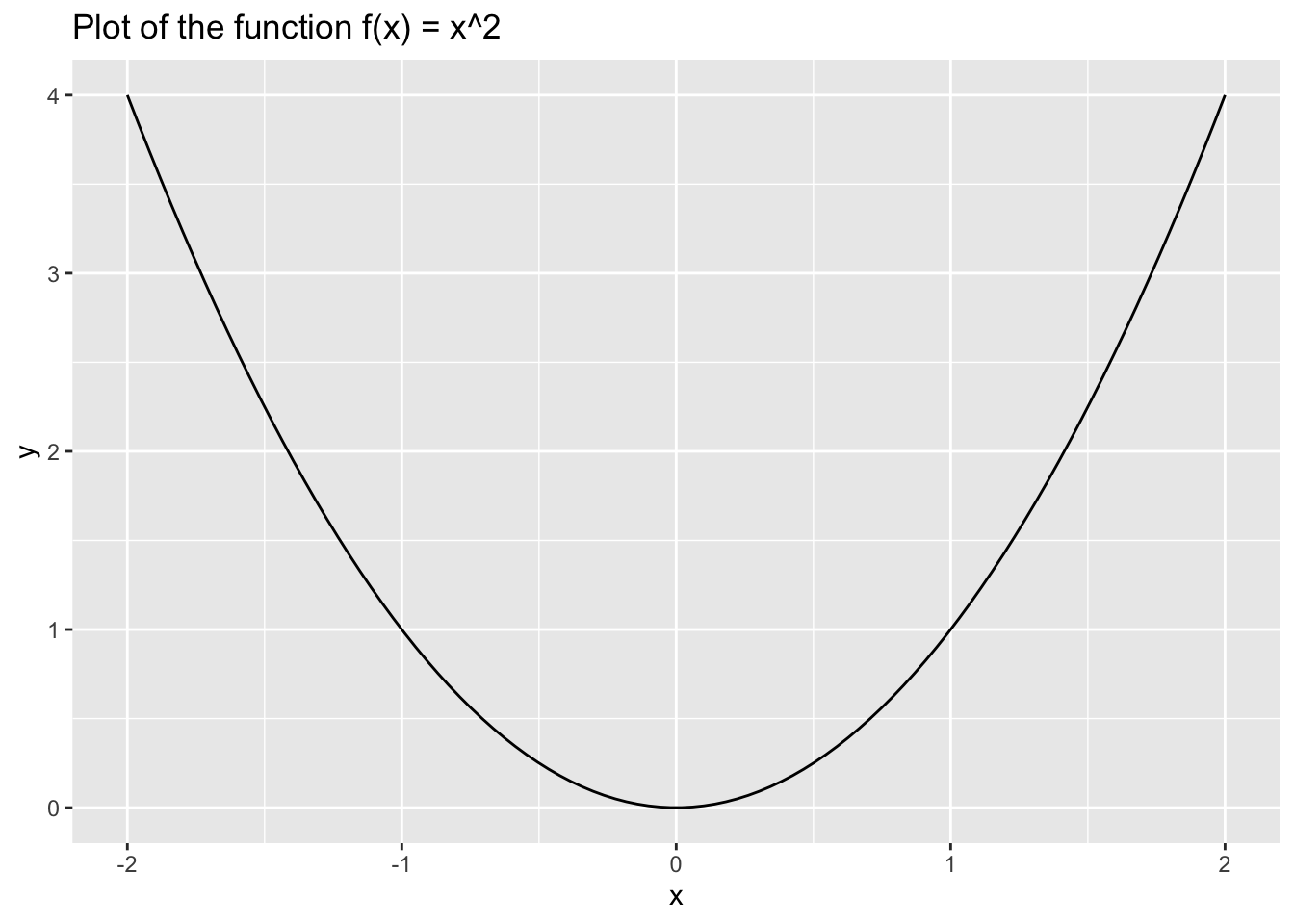

# plot the function f(x) = x^2
ggplot(data.frame(x = c(-2,2)), aes(x = x)) +
  geom_function(fun = function(x){x^2},color="steelblue",linewidth=1) +
  theme_bw(base_size=13) +
  labs(x = "x", y = "y", title = TeX("Plot of the function $f(x) = x^2$"))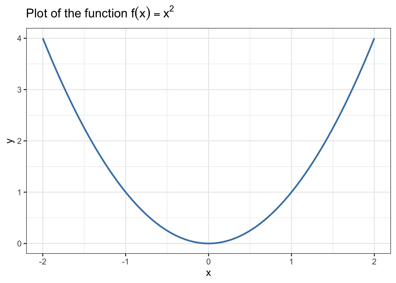

Figure 2: Plot of the function $f (x) = x^{2}$ using `geom_function` and some customizations.

# plot the functions f(x) = x^2 and g(x) = x^3
ggplot(data.frame(x = c(-2,2)), aes(x = x)) +
  geom_function(fun = function(x){x^2},aes(color="x^2"),linewidth=1) +
  geom_function(fun = function(x){x^3},aes(color="x^3"),linewidth=1) +
  theme_bw(base_size=13) +
  labs(x = "x", y = "y", title = TeX("Plot of the functions $f(x) = x^2$ and $g(x) = x^3$")) + 
  scale_color_manual(values = c("x^2" = "steelblue", "x^3" = "purple"),
                     labels = c(TeX("$x^2$"), TeX("$x^3$")))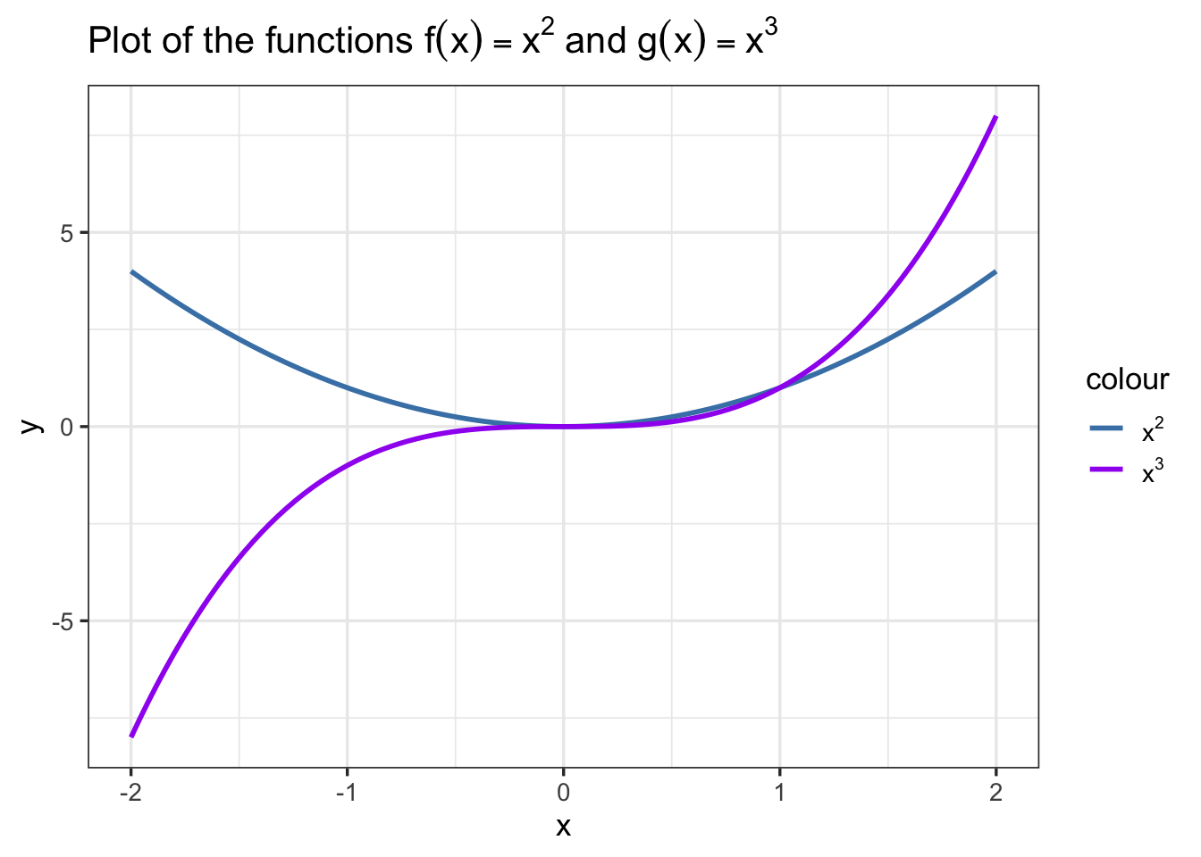

Figure 3: Plot of the functions $f (x) = x^{2}$ and $g (x) = x^{3}$ on same axes.

# plot the functions f(x) = x^2 and g(x) = x^3
p_1 <- ggplot(data.frame(x = c(-2,2)), aes(x = x)) +
  geom_function(fun = function(x){x^2},color="steelblue",linewidth=1) +
  theme_bw(base_size=13) +
  labs(x = "x", y = "y", title = TeX("Plot of the function $f(x) = x^2$"))

p_2 <- ggplot(data.frame(x = c(-2,2)), aes(x = x)) +
  geom_function(fun = function(x){x^3},color="purple",linewidth=1) +
  theme_bw(base_size=13) +
  labs(x = "x", y = "y", title = TeX("Plot of the function $g(x) = x^3$"))

p_1 + p_2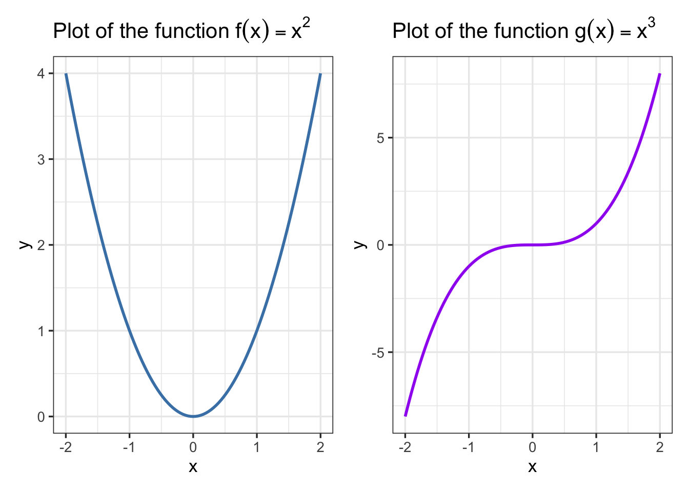

Figure 4: Plots of the functions $f (x) = x^{2}$ and $g (x) = x^{3}$ .

Intro to ggplot2 YouTube video, watch video on YouTube.

Matrices and Linear Systems

Here’s a vector:

my_vect <- c(1,-1,1)

Here’s a matrix:

my_matrix <- matrix(c(1,0,-1,3,1,2,-1,1,2), nrow = 3, ncol = 3, byrow = TRUE)
my_matrix

     [,1] [,2] [,3]
[1,]    1    0   -1
[2,]    3    1    2
[3,]   -1    1    2

Here’s the matrix-vector product:

b_vect <- my_matrix %*% my_vect
b_vect

     [,1]
[1,]    0
[2,]    4
[3,]    0

Here’s the determinant of the matrix:

det(my_matrix)

[1] -4

Here are the eigenvalues and eigenvectors of the matrix:

eigen(my_matrix)

eigen() decomposition
$values
[1]  2.7320508  2.0000000 -0.7320508

$vectors
           [,1]       [,2]       [,3]
[1,] -0.4955722 -0.5773503  0.2361737
[2,]  0.1327882 -0.5773503 -0.8814124
[3,]  0.8583563  0.5773503  0.4090649

Here’s the solution to the linear system:

solve(my_matrix, b_vect)

     [,1]
[1,]    1
[2,]   -1
[3,]    1

Root Finding

Root finding is the process of finding one or more values $x$ such that $f (x) = 0$ ². A common application of root finding in biomathematics is to find the steady states of a dynamical system.

The rootSolve package provides a number of functions for root finding in R. The methods implemented in this package are particularly well-suited for biomathematics applications because it was developed with applications to steady-state problems in mind. Here’s an example of using the uniroot.all function to find all of the roots of the function $f (x) = x^{2} - 1$ on the interval $[- 2, 2]$ :

# load the rootSolve package
library(rootSolve)

# define the function
f <- function(x){x^2 - 1}

# find the roots
(f_roots <- uniroot.all(f, c(-2,2)))

[1] -1  1

# plot the function
ggplot(data.frame(x = c(-2,2)), aes(x = x)) +
  geom_function(fun = function(x){x^2 - 1},color="steelblue",linewidth=1) +
  geom_hline(yintercept = 0, linetype = "dashed", color = "black") +
  geom_point(data=NULL,aes(x = f_roots, y = 0), color = "purple", size = 3) +
  theme_bw(base_size=13) +
  labs(x = "x", y = "y", title = TeX("Roots of the function $f(x) = x^2 - 1$ on the interval $[-2,2]$."))

Figure 5: Roots of the function $f (x) = x^{2} - 1$ on the interval $[- 2, 2]$ .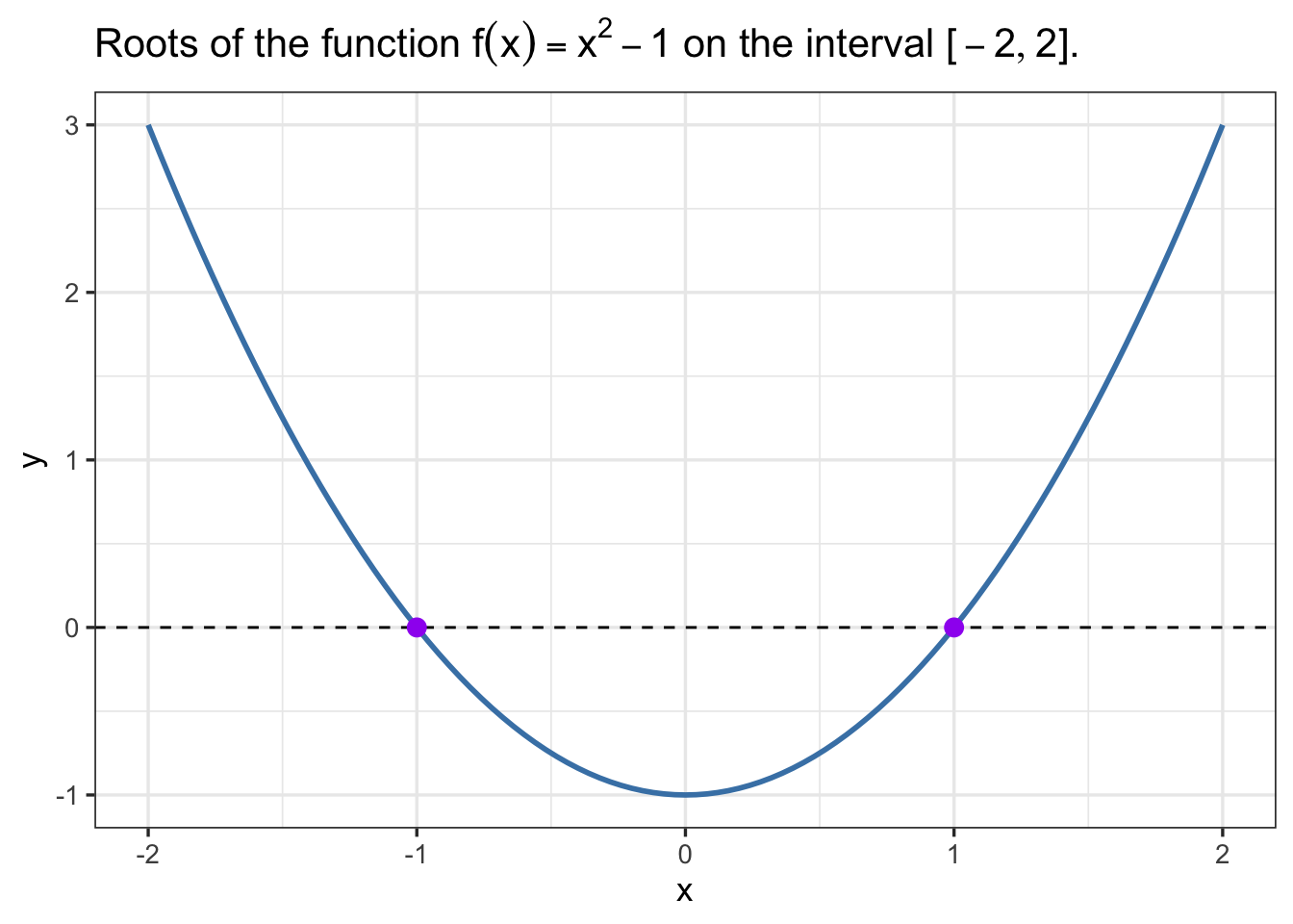

Here’s an example of using the multiroot function to find all of the roots of the system of equations $f (x, y) = (x^{2} + y^{2} - 1, x^{2} - y^{2} + 0.5)$ :

# define the function
f <- function(x) {
  c(F1 = x[1]^2+ x[2]^2 -1,
    F2 = x[1]^2- x[2]^2 +0.5)
}

# find the roots
f_roots <- multiroot(f, start = c(1,1))

# return roots
f_roots$root

[1] 0.5000000 0.8660254

Let’s check the solution:

f(f_roots$root)

          F1           F2 
2.323138e-08 2.323308e-08

The result is not exactly zero, but it’s close enough to zero that we can consider it a reasonable approximation.

Optimization

Optimization is the process of finding the extrema, that is, maximum or minimum value of a function. A common application of optimization in biomathematics is to estimate parameters for a mathematical model to fit data. One of the major challenges in such optimization problems is the potential for multiple local extrema. Here, introduce the use of basic optimization methods implemented in R. Additional details, examples, and applications will be covered in course lectures.

Base R contains the optim function for optimization, specifically minimation. However, we will utilize the extension package optimx because it unifies or streamlines the use of several optimization methods. Here’s an example of using the optimr function to find the minimum of the function $f (x) = x^{2} - 1$ on the interval $[- 2, 2]$ :

# load the optimx package
library(optimx)

# define the function
f <- function(x){x^2 - 1}

# find the minimum
f_min <- optimr(-1, f, method="L-BFGS-B",lower = -2, upper = 2)

# plot the function

ggplot(data.frame(x = c(-2,2)), aes(x = x)) +
  geom_function(fun = function(x){x^2 - 1},color="steelblue",linewidth=1) +
  geom_hline(yintercept = 0, linetype = "dashed", color = "black") +
  geom_point(data=NULL,aes(x = f_min$par, y = f_min$value), color = "purple", size = 3) +
  theme_bw(base_size=13) +
  labs(x = "x", y = "y", 
       title = TeX("Minimum of the function $f(x) = x^2 - 1$ on the interval $[-2,2]$."))

Warning in geom_point(data = NULL, aes(x = f_min$par, y = f_min$value), : All aesthetics have length 1, but the data has 2 rows.
ℹ Did you mean to use `annotate()`?

Figure 6: Minimum of the function $f (x) = x^{2} - 1$ on the interval $[- 2, 2]$ .

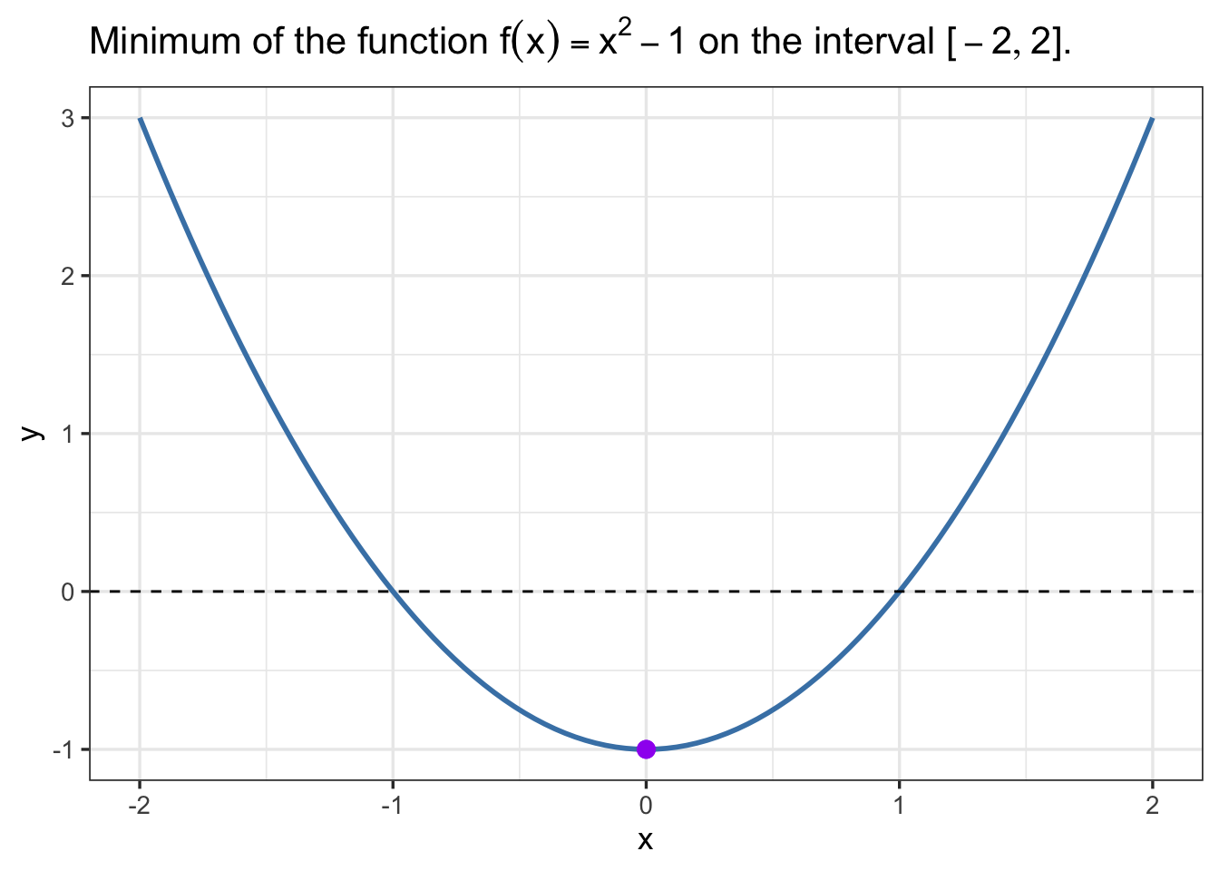
Here’s an example of using the optimr function to find the minimum of the function $f (x, y) = x^{2} + y^{2} - 1$ :

# define the function
f <- function(x) {
  return(x[1]^2+ x[2]^2 -1)
}

# find the minimum
f_min <- optimr(c(1,1), f, method="L-BFGS-B")

# return minimum
f_min$par

[1] 7.049916e-15 7.049916e-15
attr(,"status")
[1] " " " "

Differential Equations and Dynamical Systems

In this section, we provide an overview and links to detailed examples of the numerical solution of initial value problems (IVPs) for ordinary differential equations (ODEs). Additionally, the linked examples illustrate computations and visualizations of the phase plane and phase portraits for systems of ODEs. For the numerical solution of ODEs, we will use the deSolve package. For the phase plane and phase portrait computations and visualizations, we will use the phaseR package.

Briefly, most implementations of numerical methods for IVPs for ODEs require the user to define a function that returns the value of the derivative of the solution at a given time, that is, the right hand side of the ODEs. Further, the user must specify an initial condition, a time interval over which to solve the ODEs, and the values of any parameters.

View webpage with basic examples

Partial Differential Equations

Partial differential equations (PDEs) generalize ordinary differential equations (ODEs) to allow for solutions that are functions of two or more variables. Typically, in the context of biomathematics, the variables represent time and spatial coordinates. Thus, PDEs allow us to model how a biological systems change in both time and space. The examples we will see in this course will mostly be convection-diffusion type equations or systems of such equations. These PDEs have the form

$\frac{\partial c}{\partial t} = \nabla \cdot (D \nabla c - v c) + R$

Special cases include diffusion equations of which the heat equation

$\frac{\partial c}{\partial t} = D \nabla^{2} c$

is a special case. In one dimension, the heat equation is

$\frac{\partial c}{\partial t} = D \frac{\partial^{2} c}{\partial x^{2}}$

Often, in order to have a complete model, we need to specify both initial conditions and boundary conditions for the PDE problem. For example in the case of the one-dimensional heat equation, we might specify the initial temperature distribution $c (x, 0)$ and the values of the flux at the boundaries, that is $\frac{\partial c}{\partial x} (0, t)$ and $\frac{\partial c}{\partial x} (L, t)$ for $t > 0$ .

There are many approaches to the numerical solution of PDEs. We will focus on the method of lines which discretizes the spatial domain and then uses ODE solvers such as those we previously described to solve the resulting system of ODEs.

For R, the ReacTran package is available to facilitate the implementation of the method of lines for PDEs. The following links illustrate the use of this package:

Numerical solution of the heat equation in R - this page demonstrates using the ReacTran package to obtain and visualize numerical solutions for the heat equation in one dimension.

Random Variables

While MATH 463 primarily focuses on deterministic models, stochastic models are also important in biomathematics, see for example (Allen 2011). We won’t cover stochastic models in the course but will have a few occasions where it will be useful to add some stochasticity to a deterministic model. Many different probability distributions are available in R. Primarily, we focus on sampling from a distribution and accessing the probability density or probability mass function for a distribution. Further, we will demonstrate the main functions for the normal distribution and the binomial distribution. Working with other distributions is handled similarly. Additional details, examples, and applications will be covered in course lectures.

For every distribution that is implemented in R, there are four functions that can be used to access the distribution:

d<dist>: the probability density function (PDF) for continuous distributions or the probability mass function (PMF) for discrete distributions
p<dist>: the cumulative distribution function (CDF), which is the integral of the PDF or PMF
q<dist>: the quantile function, which is the inverse of the CDF
r<dist>: a random number generator (RNG) that samples from the distribution

Binomial Distributions

Recall that a binomial distribution is a discrete probability distribution that models the number of successes in a sequence of $n$ independent experiments, each asking a yes–no question, and each with its own Boolean-valued outcome: success/yes/true/one (with probability $p$ ) or failure/no/false/zero (with probability $q = 1 - p$ ). A single success/failure experiment is also called a Bernoulli trial or Bernoulli experiment and a sequence of outcomes is called a Bernoulli process; for a single trial, i.e., $n = 1$ , the binomial distribution is a Bernoulli distribution. The probability of outcomes for a binomial random variable are given by the binomial probability mass function for:

$f (k, n, p) = Pr (k; n, p) = Pr (X = k) = (\binom{n}{k}) p^{k} (1 - p)^{n - k}$

where $k$ is the number of successes, $n$ is the number of trials, and $p$ is the probability of success in each trial.

Let’s generate a random sample from a binomial distribution with $n = 10$ and $p = 0.5$ :

rbinom(5,10,0.5)

[1] 5 7 4 3 3

Let’s generate a large number of samples and plot a histogram of the results, see Figure 7.

# plot histogram
tibble(x=rbinom(1000,10,0.5)) |>
ggplot(aes(x = x)) +
  geom_histogram(binwidth = 1, color = "black", fill = "steelblue") +
  annotate("text", x = 8, y = 200, label = TeX("$n=10, p=0.5$"), size = 5) +
  theme_bw(base_size=13) +
  labs(x = "x", y = "Count", 
       title = "Binomial Distribution Samples")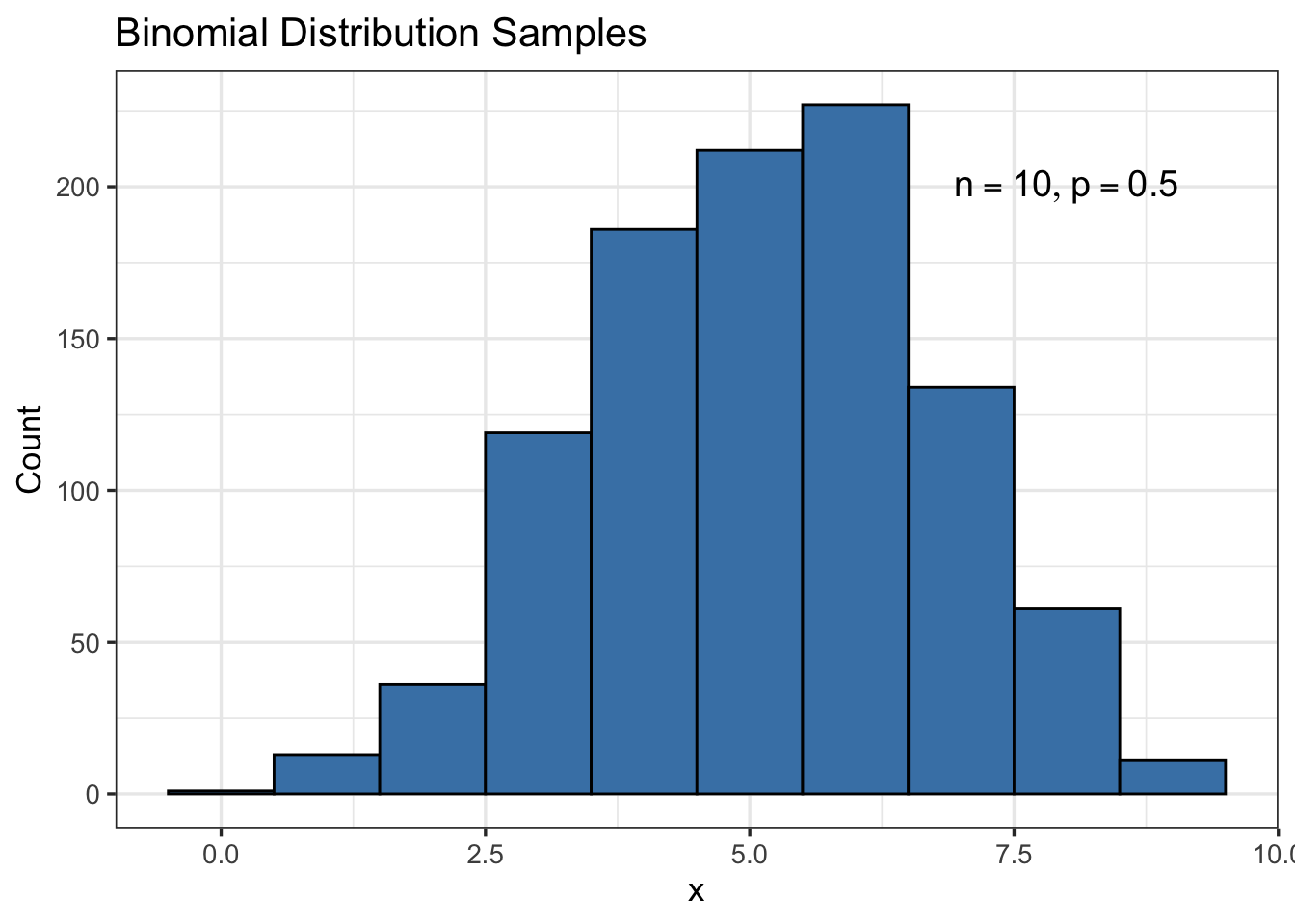

Figure 7: Histogram of 1000 samples from a binomial distribution with $n = 10$ and $p = 0.5$ .

We can work with the probability mass function as follows:

dbinom(4,10,0.5)

[1] 0.2050781

Figure 8 displays the probability mass function for a binomial random variable with $n = 10$ and $p = 0.5$ .

# plot pmf
tibble(x=0:10) |>
ggplot(aes(x = x, y = dbinom(x,10,0.5))) +
  geom_bar(stat = "identity", fill = "steelblue") +
  annotate("text", x = 9, y = 0.2, label = TeX("$n=10, p=0.5$"), size = 5) +
  theme_bw(base_size=13) +
  labs(x = "Number of Successes", y = "Probability", 
       title = "Binomial Distribution PMF")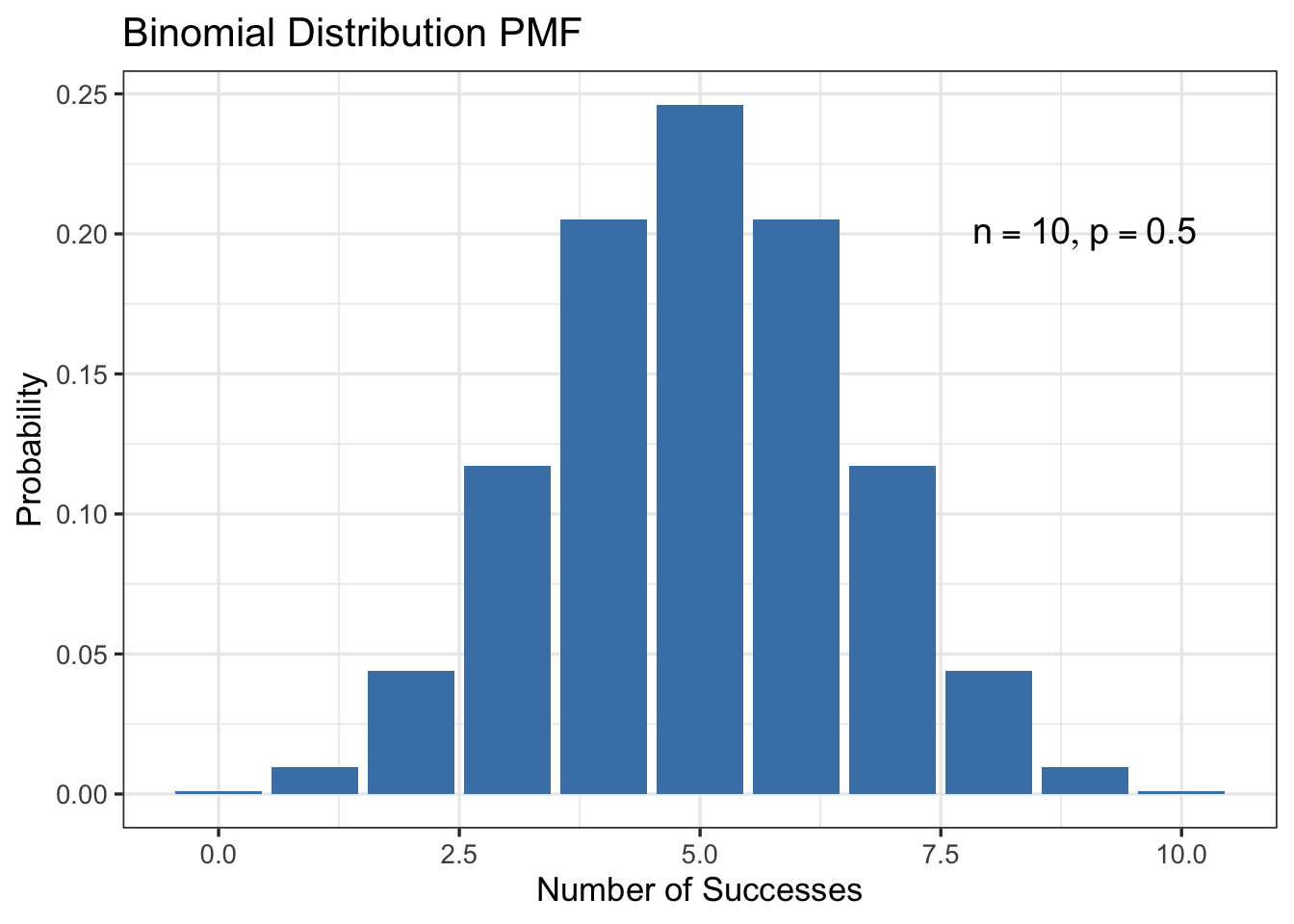

Figure 8: Probability mass function for a binomial random variable with $n = 10$ and $p = 0.5$ .

Normal Distributions

Recall that a normal distribution is a continuous probability distribution that is symmetric about the mean, showing that data near the mean are more frequent in occurrence than data far from the mean. In graph form, normal distribution will appear as a bell curve. Normal distributions are extremely important in statistics and are often used in the natural and social sciences to represent real-valued random variables whose distributions are not known. A random variable with a Gaussian distribution is said to be normally distributed and is called a normal deviate. The probability that a normal random variable with mean $μ$ and variance $σ^{2}$ has a value between $a$ and $b$ is given by the definite integral of a normal density function defined by:

$f (x ∣ μ, σ^{2}) = \frac{1}{\sqrt{2 π σ^{2}}} \exp (- \frac{(x - μ)^{2}}{2 σ^{2}})$

The parameter $σ$ is called the standard deviation.

Let’s generate a random sample from a normal distribution with $μ = 5$ and $σ = 1.5$ :

rnorm(10,5,1.5)

 [1] 2.102162 4.831484 8.070078 6.516743 3.859589 1.692009 5.242060 4.156023
 [9] 6.459276 3.127634

Let’s generate a large number of samples and plot a histogram of the results, see Figure 9.

# plot histogram
tibble(x=rnorm(1000,5,1.5)) |>
ggplot(aes(x = x)) +
  geom_histogram(binwidth = 1, color = "black", fill = "steelblue") +
  annotate("text", x = 9, y = 200, label = TeX("$\\mu=5, \\sigma=1.5$"), size = 5) +
  theme_bw(base_size=13) +
  labs(x = "x", y = "Count", 
       title = "Normal Distribution Samples")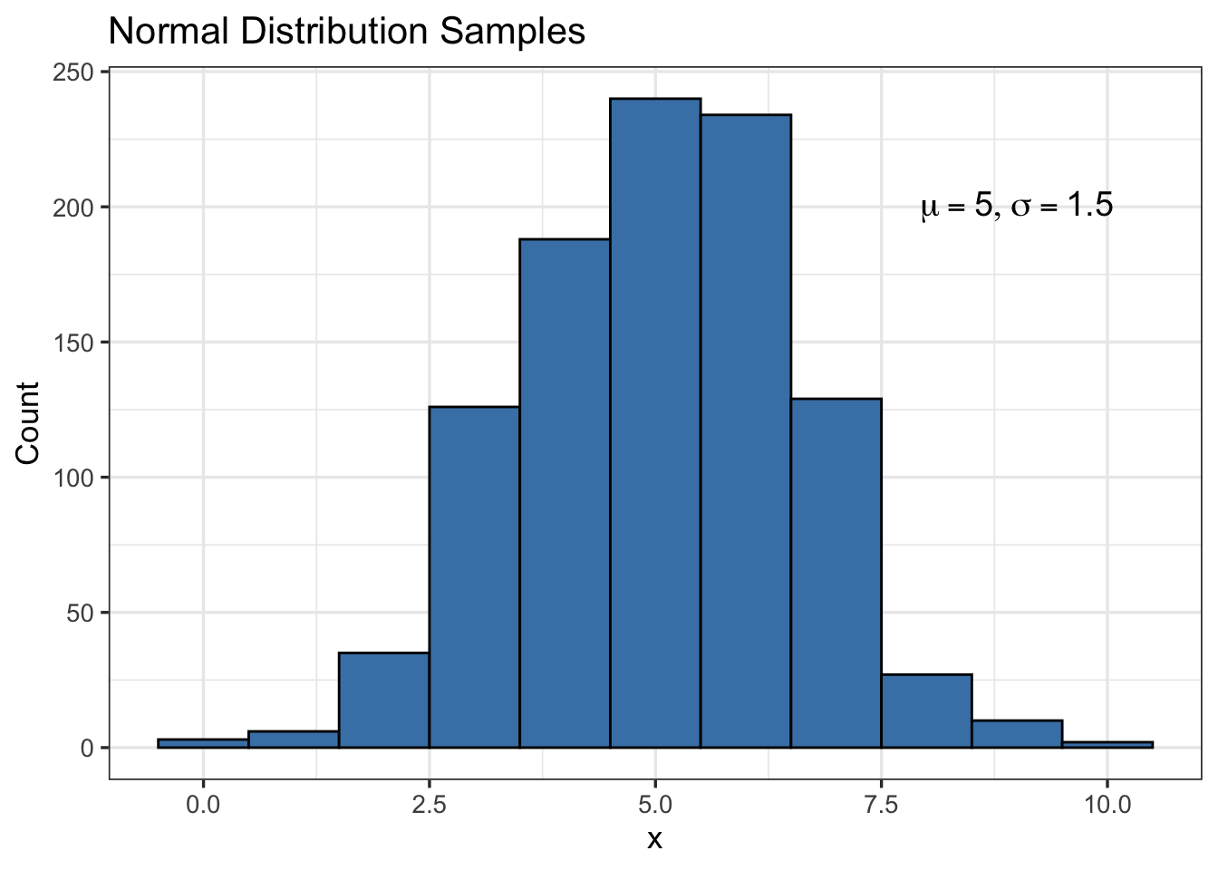

Figure 9: Histogram of 1000 samples from a normal distribution with $μ = 5$ and $σ = 1.5$ .

Next, let’s plot the probability density function for a normal distribution with $μ = 5$ and $σ = 1.5$ , see Figure 10.

# plot pdf
tibble(x=c(0,10)) |>
ggplot(aes(x = x)) +
  geom_function(fun=function(x){dnorm(x,5,1.5)},color = "steelblue",linewidth=1) +
  annotate("text", x = 9, y = 0.2, label = TeX("$\\mu=5, \\sigma=1.5$"), size = 5) +
  theme_bw(base_size=13) +
  labs(x = "x", y = "Probability", 
       title = "Normal Distribution PDF")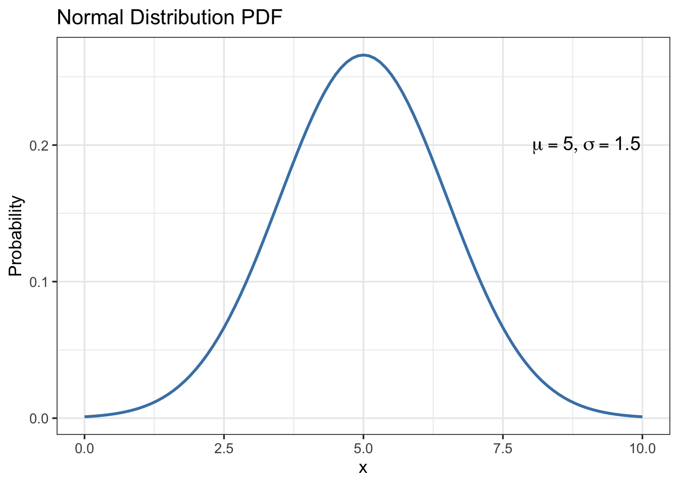

Figure 10: Probability density function for a normal distribution with $μ = 5$ and $σ = 1.5$ .

For a random variable $X \sim Norm (μ = 5, σ = 1.5)$ , the probability that $X$ is between $3$ and $7$ is given by:

$P (3 \leq X \leq 7) = \int_{3}^{7} \frac{1}{\sqrt{2 π \cdot {1.5}^{2}}} \exp (- \frac{(x - 5)^{2}}{2 \cdot {1.5}^{2}}) d x$

which we can compute in R using:

pnorm(7,5,1.5) - pnorm(3,5,1.5)

[1] 0.8175776

Thus, the area under the normal density curve with $μ = 5$ and $σ = 1.5$ between $3$ and $7$ is about 0.82.

Symbolic Math

Compared with other programming languages, R is not particularly well-suited for symbolic math. However, there are packages that can be used to perform symbolic math in R , for example:

Ryacas package for symbolic math in R.

Another option is to use the reticulate package to interface with Python and use the sympy package for symbolic math in Python. Use of the sympy package is demonstrated in the Python for Biomath tab of the course website.

References

Allen, Linda J. S. 2011. An Introduction to Stochastic Processes with Applications to Biology. Second. CRC Press, Boca Raton, FL. https://mathscinet.ams.org/mathscinet-getitem?mr=2560499.

Grayling, Michael J. 2014. “phaseR: An R Package for Phase Plane Analysis of Autonomous ODE Systems.” The R Journal 6 (2): 43–51. https://doi.org/10.32614/RJ-2014-023.

Karline Soetaert. 2009. rootSolve: Nonlinear Root Finding, Equilibrium and Steady-State Analysis of Ordinary Differential Equations.

Karline Soetaert, Thomas Petzoldt, and R. Woodrow Setzer. 2010. “Solving Differential Equations in R: Package deSolve.” Journal of Statistical Software 33 (9): 1–25. https://doi.org/10.18637/jss.v033.i09.

R Core Team. 2023. R: A Language and Environment for Statistical Computing. Vienna, Austria: R Foundation for Statistical Computing. https://www.R-project.org/.

Soetaert, Karline, and Filip Meysman. 2012. “Reactive Transport in Aquatic Ecosystems: Rapid Model Prototyping in the Open Source Software r.” Environmental Modelling & Software 32: 49–60.

Wickham, Hadley. 2016. Ggplot2: Elegant Graphics for Data Analysis. Springer-Verlag New York. https://ggplot2.tidyverse.org.

Wickham, Hadley, Mara Averick, Jennifer Bryan, Winston Chang, Lucy D’Agostino McGowan, Romain François, Garrett Grolemund, et al. 2019. “Welcome to the tidyverse.” Journal of Open Source Software 4 (43): 1686. https://doi.org/10.21105/joss.01686.

Expand for Session Info

─ Session info ───────────────────────────────────────────────────────────────
 setting  value
 version  R version 4.3.3 (2024-02-29)
 os       macOS Sonoma 14.4.1
 system   aarch64, darwin20
 ui       X11
 language (EN)
 collate  en_US.UTF-8
 ctype    en_US.UTF-8
 tz       America/New_York
 date     2024-03-31
 pandoc   3.1.12.3 @ /opt/homebrew/bin/ (via rmarkdown)
 quarto   1.4.552 @ /usr/local/bin/quarto

─ Packages ───────────────────────────────────────────────────────────────────
 package     * version    date (UTC) lib source
 deSolve     * 1.40       2023-11-27 [1] CRAN (R 4.3.1)
 dplyr       * 1.1.4      2023-11-17 [1] CRAN (R 4.3.1)
 forcats     * 1.0.0      2023-01-29 [1] CRAN (R 4.3.0)
 ggplot2     * 3.5.0      2024-02-23 [1] CRAN (R 4.3.1)
 latex2exp   * 0.9.6      2022-11-28 [1] CRAN (R 4.3.0)
 lubridate   * 1.9.3      2023-09-27 [1] CRAN (R 4.3.1)
 optimx      * 2023-10.21 2023-10-24 [1] CRAN (R 4.3.1)
 patchwork   * 1.2.0      2024-01-08 [1] CRAN (R 4.3.1)
 phaseR      * 2.2.1      2022-09-02 [1] CRAN (R 4.3.0)
 purrr       * 1.0.2      2023-08-10 [1] CRAN (R 4.3.0)
 ReacTran    * 1.4.3.1    2017-08-15 [1] CRAN (R 4.3.0)
 readr       * 2.1.5      2024-01-10 [1] CRAN (R 4.3.1)
 rootSolve   * 1.8.2.4    2023-09-21 [1] CRAN (R 4.3.1)
 sessioninfo * 1.2.2      2021-12-06 [1] CRAN (R 4.3.0)
 shape       * 1.4.6.1    2024-02-23 [1] CRAN (R 4.3.1)
 stringr     * 1.5.1      2023-11-14 [1] CRAN (R 4.3.1)
 tibble      * 3.2.1      2023-03-20 [1] CRAN (R 4.3.0)
 tidyr       * 1.3.1      2024-01-24 [1] CRAN (R 4.3.1)
 tidyverse   * 2.0.0      2023-02-22 [1] CRAN (R 4.3.0)

 [1] /Library/Frameworks/R.framework/Versions/4.3-arm64/Resources/library

──────────────────────────────────────────────────────────────────────────────

Footnotes

Note that you must install a package before you can load it. You can install a package using the install.packages function or the Packages tab in the RStudio IDE. Packages only need to be installed once but must be loaded in each new R session.↩︎
Note that we allow for the function $f$ to be vector-valued, in which case we are looking for solutions to a system of nonlinear equations.↩︎

Reuse

CC BY-NC-SA 4.0